自省 自行 自醒

深入浅出 effective_cache_size

Word count: 2kReading time: 9 min
2024/02/19
loading

前言

关于 effective_cache_size 参数许久之前也曾翻译过一篇文章,最近在复核 14 internal 的时候,又有了一些新的理解与感触。

何如

众所周知,在 PostgreSQL 的双缓存架构下,其对于自己的 shared_buffers 有着”绝对”掌控权,但是对于文件系统缓存一无所知,加之 cache 几乎无处不在,除了文件系统,存储有、RAID 卡有、磁盘可能也有,因此优化器还要考虑到这些缓存的存在

We also use a rough estimate “effective_cache_size” of the number of disk pages in Postgres + OS-level disk cache. (We can’t simply use NBuffers for this purpose because that would ignore the effects of the kernel’s disk cache.)

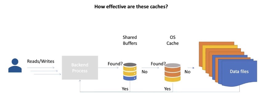
effective_cache_size 便是做这个的,简而言之,此参数用于告诉优化器有多少缓存可以用于查询,包括操作系统的缓存,按照一般经验,推荐设置为 RAM * 0.7

Sets the planner’s assumption about the effective size of the disk cache that is available to a single query.

然而官网的解释比较粗糙,其详细原理并没有过多阐述,只是给出了如何调整的建议,越高越可能使用索引,越低则倾向于使用顺序扫描。

This is factored into estimates of the cost of using an index; a higher value makes it more likely index scans will be used, a lower value makes it more likely sequential scans will be used

更高的数值会使得索引扫描更可能被使用,更低的数值会使得顺序扫描更可能被使用。

让我们看看代码中的注解,深入了解其原理。代码位于 costsize.c 中

1
2
3
4
5
6
7
8
9
10
11
12
13
14
15
16
17
18
19
20
21
22
23
24
25
26
27
28
29
30
31
32
33
34
35
36
37
38
39
40
41
42
43
/*
* index_pages_fetched
* Estimate the number of pages actually fetched after accounting for
* cache effects.
*
* We use an approximation proposed by Mackert and Lohman, "Index Scans
* Using a Finite LRU Buffer: A Validated I/O Model", ACM Transactions
* on Database Systems, Vol. 14, No. 3, September 1989, Pages 401-424.
* The Mackert and Lohman approximation is that the number of pages
* fetched is
* PF =
* min(2TNs/(2T+Ns), T) when T <= b
* 2TNs/(2T+Ns) when T > b and Ns <= 2Tb/(2T-b)
* b + (Ns - 2Tb/(2T-b))*(T-b)/T when T > b and Ns > 2Tb/(2T-b)
* where
* T = # pages in table
* N = # tuples in table
* s = selectivity = fraction of table to be scanned
* b = # buffer pages available (we include kernel space here)
*
* We assume that effective_cache_size is the total number of buffer pages
* available for the whole query, and pro-rate that space across all the
* tables in the query and the index currently under consideration. (This
* ignores space needed for other indexes used by the query, but since we
* don't know which indexes will get used, we can't estimate that very well;
* and in any case counting all the tables may well be an overestimate, since
* depending on the join plan not all the tables may be scanned concurrently.)
*
* The product Ns is the number of tuples fetched; we pass in that
* product rather than calculating it here. "pages" is the number of pages
* in the object under consideration (either an index or a table).
* "index_pages" is the amount to add to the total table space, which was
* computed for us by make_one_rel.
*
* Caller is expected to have ensured that tuples_fetched is greater than zero
* and rounded to integer (see clamp_row_est). The result will likewise be
* greater than zero and integral.
*/
double
index_pages_fetched(double tuples_fetched, BlockNumber pages,
double index_pages, PlannerInfo *root)
{
...

看起来很生硬,代码看得我云里雾里。简而言之,计算采用了 Mackert 和 Lohman 提出的模型,这个方法旨在估算有限 LRU 缓冲区下索引扫描的 I/O 成本。
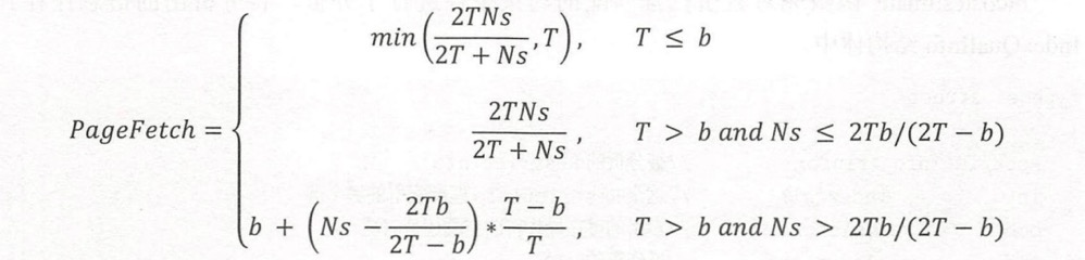
该公式基于以下参数:

  • T:表中的页面数
  • N:表中的元组数
  • s:约束条件的选择率
  • b:表上的页面已经在缓存中的数量

index_pages_fetched 通过这个公式估算,在考虑到缓存效应后,实际需要获取的页面数量。这种方法帮助优化器在考虑不同查询执行计划时,更准确地估算 I/O 成本,从而选择最佳的查询执行策略。

假设当前查询中涉及的所有表的总页面是 total_pages,effective_cache_size 表示当前查询中涉及的所有表已经加载到缓存的总页面数,那么 (细节可以参照查询优化深度探索一书):

分析

代码过于晦涩,让我们看个实际例子:

1
2
3
4
5
6
7
8
9
10
postgres=# CREATE TABLE t_ordered AS SELECT id, ceil(random() * 100000000) AS r FROM generate_series(1, 1000000) AS id;
SELECT 1000000
postgres=# analyze t_ordered ;
ANALYZE
postgres=# select attname,correlation from pg_stats where tablename = 't_ordered';
attname | correlation
---------+---------------
id | 1
r | -0.0018580947
(2 rows)

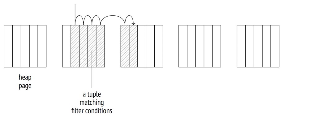
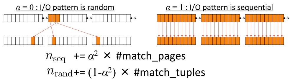
t_ordered 表的 id 列相关性为 1,表示完美关联,元组在磁盘上的物理顺序与索引中 TIDS 的逻辑顺序完美相关,那么每个页面只会被访问一次:Index Scan 节点将顺序地从一个页面跳到另一个页面,逐个读取元组。

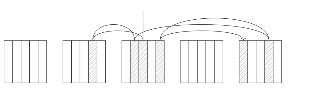
而 r 列为 0.0018,越接近 0 的值表示数据越杂乱无章,Index Scan 节点必须在页面之间跳转,而不是顺序读取;在最坏的情况下,访问的页面数量会达到获取的元组数量。

让我们粗略计算下总成本是如何计算出来的,记住前提是 id 列的相关性为 1

1
2
3
4
5
6
7
8
9
10
11
12
13
14
15
16
postgres=# create index on t_ordered(id);
CREATE INDEX
postgres=# create index on t_ordered(r);
CREATE INDEX
postgres=# analyze t_ordered ;
ANALYZE
postgres=# set enable_bitmapscan to off;
SET
postgres=# set enable_seqscan to off;
SET
postgres=# explain select * from t_ordered where id < 100000;
QUERY PLAN
------------------------------------------------------------------------------------------
Index Scan using t_ordered_id_idx on t_ordered (cost=0.42..3351.27 rows=98677 width=12)
Index Cond: (id < 100000)
(2 rows)

优化器预估返回 98677 条,那么选择率为 0.098677

1
2
3
4
5
postgres=# select 98677/reltuples as selectivity from pg_class where relname = 't_ordered';
selectivity
-------------
0.098677
(1 row)

索引扫描的成本包括:

  1. CPU cost of searching B+-tree,扫描 B 树的成本
  2. CPU cost of scanning index tuples in leaf pages,在叶子页搜索匹配元组的成本
  3. I/O cost of leaf pages,叶子页面的 I/O 成本
  4. I/O cost of heap pages,堆页面的 I/O 成本
  5. CPU cost of scanning heap tuples,扫描堆元组的成本

具体细节可以参考 https://www.interdb.jp/pg/pgsql03/02.html,此处粗略计算一下:

1
2
3
4
5
6
7
8
9
10
11
12
13
14
15
16
17
18
19
20
21
22
23
24
25
26
27
28
29
30
postgres=# WITH costs(idx_cost, tbl_cost) AS (
SELECT
(
SELECT round(
current_setting('random_page_cost')::real * pages +
current_setting('cpu_index_tuple_cost')::real * tuples +
current_setting('cpu_operator_cost')::real * tuples
)
FROM (
SELECT relpages * 0.098677 AS pages, reltuples * 0.098677 AS tuples
FROM pg_class WHERE relname = 't_ordered_id_idx'
) c
),
(
SELECT round(
current_setting('seq_page_cost')::real * pages +
current_setting('cpu_tuple_cost')::real * tuples
)
FROM (
SELECT relpages *0.098677 AS pages, reltuples * 0.098677 AS tuples
FROM pg_class WHERE relname = 't_ordered'
) c
)
)
SELECT idx_cost, tbl_cost, idx_cost + tbl_cost AS total
FROM costs;
idx_cost | tbl_cost | total
----------+----------+-------
1824 | 1524 | 3348
(1 row)

我们计算出来的结果为 3348,和优化器算出来的 3351 接近,当然这是一个近似值。现在,让我们基于随机列的查询 (返回大致相同的行数,使选择率大致相同):

1
2
3
4
5
6
postgres=# explain select * from t_ordered where r < 10000000;
QUERY PLAN
------------------------------------------------------------------------------------------
Index Scan using t_ordered_r_idx on t_ordered (cost=0.42..24555.56 rows=98071 width=12)
Index Cond: (r < '10000000'::double precision)
(2 rows)

计算方式类似,不过此处是 random 列,相关性并非 1

1
2
3
4
5
6
7
8
9
10
11
12
13
14
15
16
17
18
19
20
21
22
23
24
25
26
27
28
29
30
postgres=# WITH costs(idx_cost, tbl_cost) AS (
SELECT
(
SELECT round(
current_setting('random_page_cost')::real * pages +
current_setting('cpu_index_tuple_cost')::real * tuples +
current_setting('cpu_operator_cost')::real * tuples
)
FROM (
SELECT relpages * 0.098071 AS pages, reltuples * 0.098071 AS tuples
FROM pg_class WHERE relname = 't_ordered_r_idx'
) c
),
(
SELECT round(
current_setting('random_page_cost')::real * tuples +
current_setting('cpu_tuple_cost')::real * tuples
)
FROM (
SELECT relpages * 0.098071 AS pages, reltuples * 0.098071 AS tuples
FROM pg_class WHERE relname = 't_ordered'
) c
)
)
SELECT idx_cost, tbl_cost, idx_cost + tbl_cost AS total
FROM costs;
idx_cost | tbl_cost | total
----------+----------+--------
1812 | 393265 | 395077
(1 row)

可以看到这种方式计算出来的值和优化器算出来的相差极大,原因不难理解,优化器考虑了缓存,默认的 effective_cache_size 为 4GB。

假如我们将其设为最小值,这样计算出来的值 394988.27 就和我们计算出来的值十分接近了。

1
2
3
4
5
6
7
8
postgres=# set effective_cache_size to '8kB';
SET
postgres=# explain select * from t_ordered where r < 10000000;
QUERY PLAN
-------------------------------------------------------------------------------------------
Index Scan using t_ordered_r_idx on t_ordered (cost=0.42..394988.27 rows=98071 width=12)
Index Cond: (r < '10000000'::double precision)
(2 rows)

小结

小结一下

  1. effective_cache_size 用于告诉优化器有多少缓存可以用于查询,并非真正分配这么多,仅仅是一个参考值,当评估叶子页面的 I/O 成本时,优化器会考虑到 effective_cache_size,越大,索引扫描的成本就越低,也就越倾向于使用索引扫描
  2. 而 correlation 相关性决定了元组在磁盘上的物理顺序和逻辑顺序,也决定了堆页面的 I/O 成本,能否顺序访问的概率

参考

https://www.interdb.jp/pg/pgsql03/02.html

https://www.cybertec-postgresql.com/en/effective_cache_size-a-practical-example/

https://www.cybertec-postgresql.com/en/effective_cache_size-what-it-means-in-postgresql/

CATALOG
  1. 1. 前言
  2. 2. 何如
  3. 3. 分析
  4. 4. 小结
  5. 5. 参考